Traffic Sign Recognition
Build a Traffic Sign Recognition Project
The goals / steps of this project are the following:
- Load the data set (see below for links to the project data set)
- Explore, summarize and visualize the data set
- Design, train and test a model architecture
- Use the model to make predictions on new images
- Analyze the softmax probabilities of the new images
- Summarize the results with a written report
Rubric Points
Here I will consider the rubric points individually and describe how I addressed each point in my implementation.
Code
Here is an explanation of how I approached this project. If you want to dive in the code, it’s right here ! You’ll find that I used tf.summary. It has to do with TensofBoard, TensorFlow’s visualization tool.
Data Set Summary & Exploration
1. Dataset presentation
The data is provided in pickle files. It is already split in a training set, a validation set and a test set.
- There are 34799 images in the training set.
- There are 4410 images in the validation set.
- There are 12630 images in the test set.
- Each image is 32 by 32 pixels, each having a R,G and B component. Their shape is therefore (32, 32, 3).
- The dataset contains 43 different traffic signs. They are called classes.
2. Visualization of the dataset.
Here is an exploratory visualization of the data set. Each label (type of traffic sign) displays an example of its class underneath it.

Right away, we can see that not all these images are great. For example, I absolutely couldn’t tell what is the traffic sign of the labels 13, 15, 19 and 38 if it wasn’t written next to it ! We’ll find a solution …
It is a bar chart showing how the data is shared across the different classes and sets.

We can see that there is some great disparity among the different classes. The most represented one contains 2010 images whereas the smallest one contains only 180.
Design and Test a Model Architecture
1. Image preprocessing
From what I seen in papers, people tend to remove the color components and convert the image to greyscale. I believe that the color is helpful so I decided to keep the R, G and B channels. I later tried to convert the images to greyscale before training the network but didn’t obtain any significant improvement.
ROI Cropping
For each image of each dataset, a region of interest is provided. It gives a precise location to where the sign actually is. In order to maximize my chances that the model is going to learn features from the sign I crop the background to remove the noise as much as possible.

Normalization
What is recommended to do is to center the data so it has 0 mean. Instead, I remove 180 to each RGB channels. It is very similar and would perform well for my model. I normalized the scale of each image to range between -1 and 1. This allows a better convergence of the model because the computation of the gradient is facilitated.

It is important to note that the normalization needs to be applied to every set (training, validation et test sets) in order to train a working model.
Due to the disparity between classes and the total numbers of images in the training data, I decided to augment the dataset.
To augment the dataset means to add new training data. Copy identically data from the training set is not a good idea because it increases the risk of overfitting. The goal is to take images from the training set and modify them a little bit so that it presents new features but still belonging to the same class.
In order to do so, I created 2 functions.
Rotation
The first idea is to rotate the image a little bit. The angle is determined randomly and bounded between -15° and +15°. It wouldn’t make sense to rotate them more than that since the car would never see traffic sign that are upside down. It is worth noticing that it could be interesting to do so for another dataset like classify galaxies! for example.
Here is an example of my random rotation function:

Stretching
Lastly, from the observation made that the car is not always facing the traffic sign, the model must therefore be able to classify the sign even if this one presents some distortion.
Here comes an example of my random stretching function and the comparison with an non-stretched image.

With this set of augmenting functions defined. I could start augmenting the dataset for real.
Here is when I started struggling. I spent a huge amount of time trying to figure out what I was doing wrong. The kernel kept crashing. Lesson learned. Do not develop in a Jupyter Notebook.
2. Model architecture.
My final model consisted of the following layers:
| Layer | Description |
|---|---|
| Input | 32x32x3 RGB image |
| Convolution 5x5 | 1x1 stride, VALID padding, outputs 28x28x6 |
| RELU | |
| Max pooling | 2x2 stride, outputs 14x14x6 |
| Convolution 5x5 | 1x1 stride, VALID padding, outputs 10x10x16 |
| RELU | |
| Max pooling | 2x2 stride, outputs 5x5x6 |
| Flatten | outputs 400 |
| Fully connected | outputs 120 |
| RELU | |
| Dropout | probability = 0.5 |
| Fully connected | outputs 84 |
| RELU | |
| Dropout | probability = 0.5 |
| Fully connected | outputs 43 |
| Softmax |
Dropout
Dropout is relatively recent regularization technique used to avoid overfitting. During training, we let every neuron propagate its output with a probability dropout or set it to 0 otherwise. When backpropagation is performed, only the neurons activated end up having their weights updated.
The idea behind the concept is that since sometimes some connections are missing, the model can’t rely/focus on an irrelevant signals. It could be seen as training the model on an exponential number of “thinned” networks with extensive weight sharing.
Let’s not forget to set the dropout probability (effectively being the probability to keep the output connection of a neuron active) to 1 when we want to validate/test out model with the validation/test sets or when we want to predict the class of a new image to obtain the average of all of these “thinned” networks.

Image taken from the dropout paper.
3. Describe how you trained your model. The discussion can include the type of optimizer, the batch size, number of epochs and any hyperparameters such as learning rate.
Adam Optimizer
Adam offers several advantages over the simple tf.train.GradientDescentOptimizer. Foremost is that it uses moving averages of the parameters. The concept behind this is called “momentum”. The provided learning rate is the maximum coefficient applied to the gradient during backpropagation. The Adam optimizer determines when to lower that learning rate for each parameter. This brings some computation overhead as this is performed for each training step (maintain the moving averages and variance, and calculate the scaled gradient). A simple tf.train.GradientDescentOptimizer could equally be used in your MLP, but would require more hyperparameter tuning before it would converge as quickly.
4. Describe the approach taken for finding a solution and getting the validation set accuracy to be at least 0.93. Include in the discussion the results on the training, validation and test sets and where in the code these were calculated. Your approach may have been an iterative process, in which case, outline the steps you took to get to the final solution and why you chose those steps. Perhaps your solution involved an already well known implementation or architecture. In this case, discuss why you think the architecture is suitable for the current problem.
If an iterative approach was chosen:
- What was the first architecture that was tried and why was it chosen?
- What were some problems with the initial architecture?
- How was the architecture adjusted and why was it adjusted? Typical adjustments could include choosing a different model architecture, adding or taking away layers (pooling, dropout, convolution, etc), using an activation function or changing the activation function. One common justification for adjusting an architecture would be due to overfitting or underfitting. A high accuracy on the training set but low accuracy on the validation set indicates over fitting; a low accuracy on both sets indicates under fitting.
- Which parameters were tuned? How were they adjusted and why?
- What are some of the important design choices and why were they chosen? For example, why might a convolution layer work well with this problem? How might a dropout layer help with creating a successful model?
If a well known architecture was chosen:
- What architecture was chosen?
- Why did you believe it would be relevant to the traffic sign application?
- How does the final model’s accuracy on the training, validation and test set provide evidence that the model is working well?
At first, I started with the LeNet-5 architecture from the lesson. It is known to be one of the very first Convolutionnal Neural Network to lower the error rate significantly for the MNIST dataset. I thought it would be a good model to try.
Here is where I kept my observations from the early tests. I use the acronym VA for Validation Accuracy, LR for Learning Rate, BS for Batch Size, DO for Dropout. With the LeNet-5 NN from the lecture, the validation accuracy barely reached over 85%. One of the first improvement I’ve made was to add a dropout unit to prevent from overfitting.
I reached 86.3% with 1 dropout unit and a dropout input argument of 0.7. I reached 87.9% with 2 dropout unit and a dropout input argument of 0.7.
The idea I had was to reduce the learning rate a little bit and increase the number of epochs.
With 20 epochs, LR = 0.001: 1. Batch size of 64, VA = 90.6% 2. Batch size of 128, VA = 88.9%
It would seem like reducing the batch size would improve the accuracy but a larger batch size requires a smaller learning rate.
Then I added the normalization of the rgb components to be between 0.1 and 0.9 instead of 0, 255.
With 20 epochs, BS = 128: 1. LR = 0.0005, VA = 90.1% 2. LR = 0.001, VA = 90.4%
No great conclusion could be drawn with this experiment.
Then I augmented the images by cropping them to only keep the region of interest. I obtained the following results with a batch size of 128 images, a LR = 0.0005 and 20 epochs. 1. D0 = 1, VA = 92.5% (No Dropout) 2. D0 = 0.7, VA = 95.3% (Dropout x2 only after fully connected layers.) 3. D0 = 0.7, VA = 94.4% (Dropout x4 after each ReLU.)
I concluded that I should only keep the dropout cells after the activation of the fully connected layers. Furthermore, cropping the image is impacting the result of the neural network by a lot.
I was pretty happy with my early results using the LeNet-5 network architecture so I haven’t jumped to another one but rather focus on fine tuning the parameters on this model.
I wanted to tune the dropout parameter. Here are 2 graphs displaying the evolution of the loss and accuracy for both the training set and the validation set at each epoch during training.
For the same hyperparameters and the dropout set to 0.7:

Then I changed it to be 0.5:

Then, I started to include my rotating augmenting function. Therefore, I increased the size of the training set. With now 39239 training images, BS = 128, LR = 0.0005, Epochs = 50, DO = 0.7, I obtained a validation accuracy of 99.9% and a training accuracy of 96.6%. Unfortunately, I believe I overfitted the model because the test accuracy was only 65%.
In the end, after tweaking the parameters I finally ended up with this solution: Number of epochs : 20 Batch size : 128 Learning rate : 0.0005 Dropout : 0.5 Training Accuracy = 99.023% Validation Accuracy = 95.170% Test accuracy = 69.4%.
Test of my model on New Images
1. Presentation of the images
Here are 16 images from the Belgium traffic sign dataset:
Theses images have the same meaning that the ones of the German dataset but some might have some small differences like of example the presence of km/h on the 50 km/h speed limit sign or the width of some arrows. Other that that, these images do not present major problems of visibility that might trick the model but in order to perform well on these images, it comes down to how good were the images of the training data. I want to highlight here that I believe that these images were not very clear. I had a hard time determining the class of many of the images in the dataset myself.
2. Predictions labels of these images and their top 5 softmax probabilities
Here are the results of the prediction:
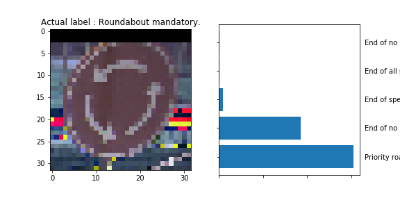
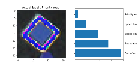
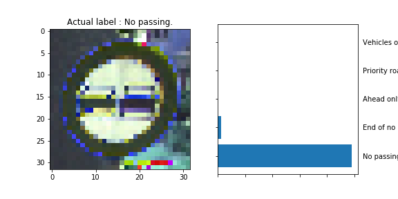
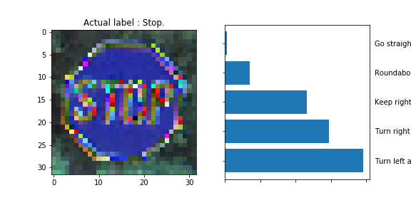
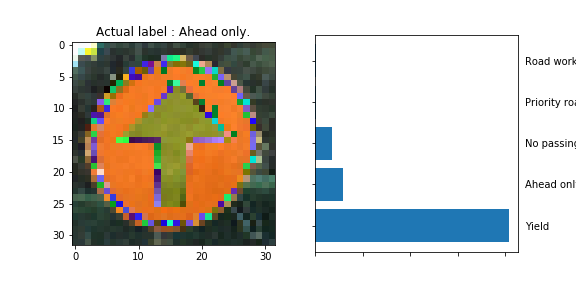
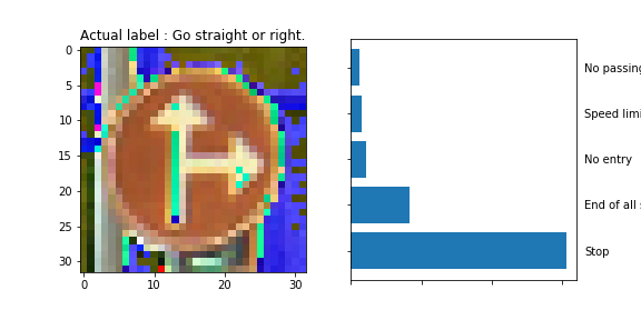
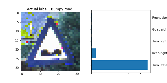
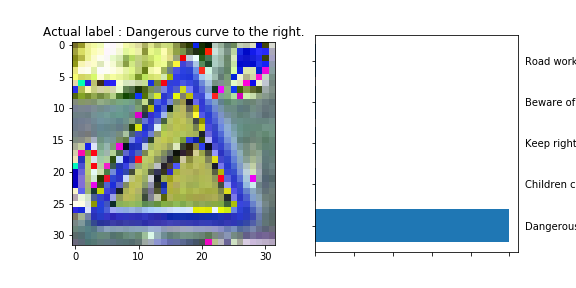
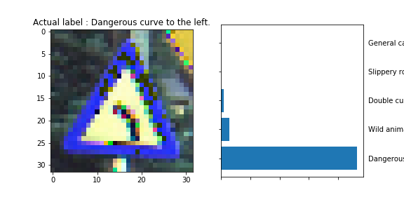
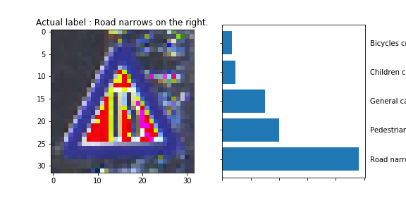
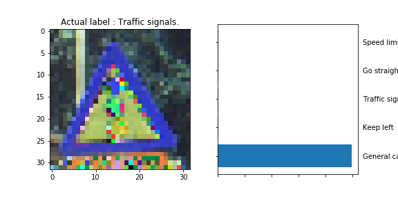
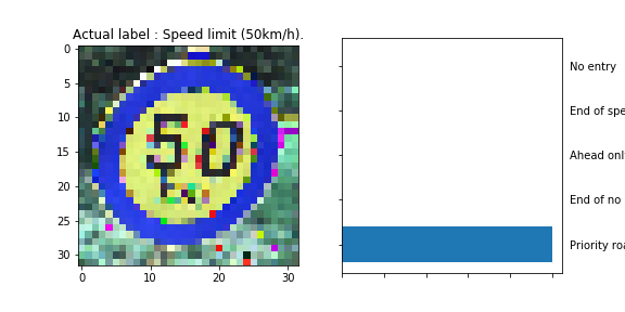
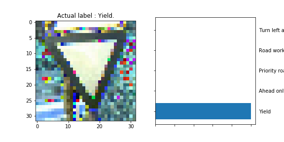
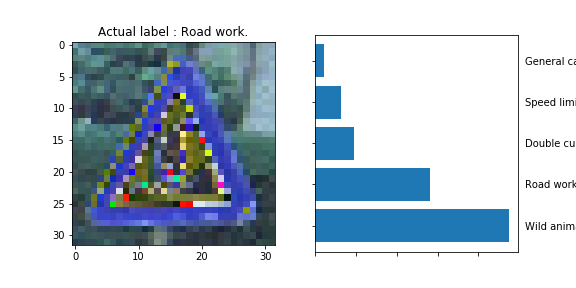
The model was able to correctly guess 8 of the 15 traffic signs, which gives an accuracy of 53%. This compares unfavorably to the accuracy on the test set of 70%.
We can interpret some of the results and make some assumptions.
-
Roundabout mandatory: The circular gap between the 3 arrows and the border of the sign could have been interpreted as the yellow border of the Priority Road sign and therefore misclassified.
-
The dangerous curve to the left is somehow resemblant to the Slippery Slope Road sign.
-
The General Caution sign exhibits a very similar vertical pattern to the one present on the Traffic Signals sign.
-
The
5in the 50 km/h sign is very similar to the6in the 60 km/h sign and must have caused the misclassification. -
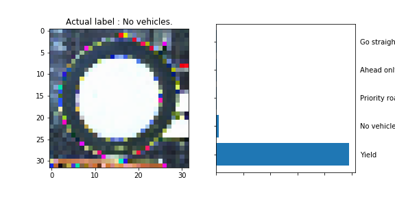
The Yield sign’s output neuron has probably learned to fire a high output when a significant area in the middle of the image is white (or of uniform color/intensity) rather than focusing on the shape of the sign. The might by why the
No Vehiclesign was classified as being aYieldsign.