Behavioral Cloning

Behavioral Cloning Project

The goals / steps of this project are the following:

• Use the simulator to collect data of good driving behavior
• Build, a convolution neural network in Keras that predicts steering angles from images
• Train and validate the model with a training and validation set
• Test that the model successfully drives around track one without leaving the road
• Summarize the results with a written report

Rubric Points

Here I will consider the rubric points individually and describe how I addressed each point in my implementation.

Files Submitted & Code Quality

1. Submission includes all required files and can be used to run the simulator in autonomous mode

My project includes the following files:

• clone.py containing the script to create and train the model
• drive.py for driving the car in autonomous mode
• model.h5 containing a trained convolution neural network
• writeup_report.md or writeup_report.pdf summarizing the results

2. Submission includes functional code

Using the Udacity provided simulator and my drive.py file, the car can be driven autonomously around the track by executing

python drive.py model.h5

3. Submission code is usable and readable

• The clone.py file contains the code for training and saving the convolution neural network.
• The augmenting and preprocessing pipeline I used for training and validating the model is in data.py, and it contains comments to explain how the code works.
• I perform some tests in test.py. The code in that file allowed me to output the figures in this report.

The code has been separated for clarity.

Model Architecture

1. Models Experimented

In this case, I needed a regression network that outputs a unique output, the steering angle. This result is then used to steer the car.

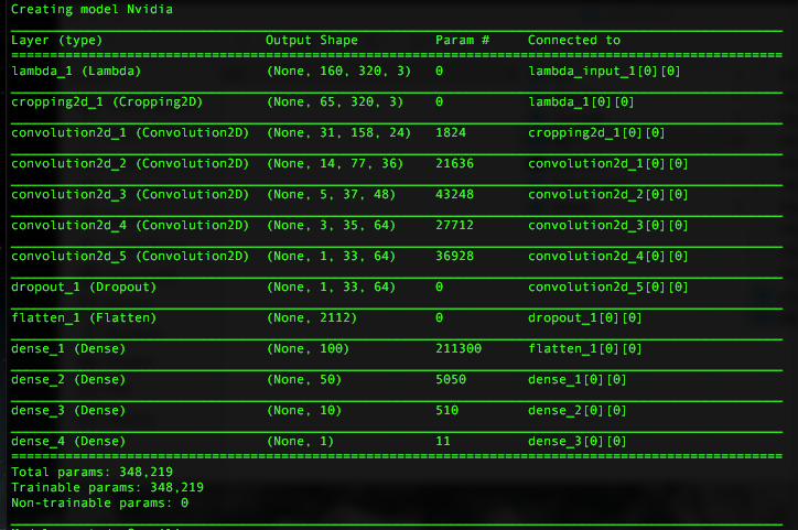
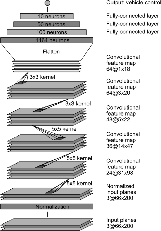
I have been really impressed by the work Nvidia has been doing using convolutional neural network to teach a car how to drive by itself by copying the driving habits of a human driver as described in this paper.

The Nvidia model consists of a convolution neural network with 3x3 filter sizes and depths between 24 and 64.

• First, I added a lambda layer to normalize the image between -0.5 and 0.5.
• I use the cropping function provided by keras to remove the parts of the image that are not relevant (70 pixels at the top and 25 pixels at the bottom of the image, keep the full width).
• The rest of the model is the same as used by nvidia accept that my input image is not the same as theirs.
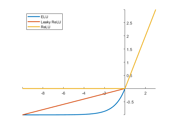
• The model includes ELU layers to introduce nonlinearity.

On the other hand, George Hotz and his company Comma.ai have achieved groundbreaking results before releasing the architecture of their CovNet. I tested their model as well.

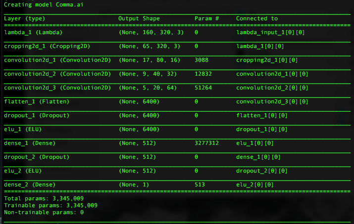
We can note that the Comma.ai model trains 10 times more parameters compared to the one used by Nvidia.

2. Attempts to reduce overfitting in the model

Both models contain dropout layers in order to reduce overfitting.

The model was trained and validated on different data sets to ensure that the model was not overfitting. In that case, it doesn’t make sense to keep a set of the data dedicated for testing. The model was tested by running it through the simulator and ensuring that the vehicle could stay on the track.

3. Model parameter tuning

Both model used an adam optimizer, so the learning rate was not tuned manually.

Training Strategy

1. Appropriate training data

At first, I drove the car with the arrows of the keyboard. This creates very unevenly distributed data which can’t be, I believe, further from the reality. I rapidly changed to driving the car with my trackpad which turned out to provide very smooth steering angles.

I drove the car in the center of the road as accurately as possible for 2 laps. I also added some recovery data, recordings where the car happen to be on the side of the road and steer back to the center of the road. I found that process tricky because the by doing so, the car can learn from bad data.

After testing I found out that the training data with which I first succeeded to close an autonomously driven gap on the first track was the following:

• 4 laps where the vehicle is driving in the center of the road.
• Recovering from the left and right sides of the road was not recorded.

2. Data presentation

Here are the 3 images that are generated by the simulation software provided by Udacity at any given time:

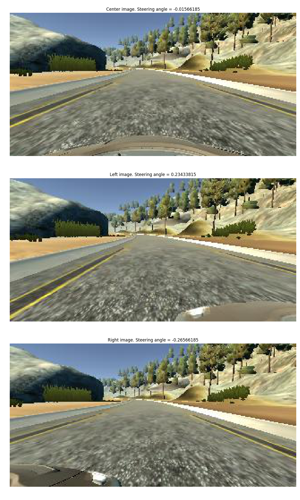
The steering angle of the first image is the one recorded. I then derive the steering angle to be applied for the left and right cameras.

3. Preprocessing pipeline

The preprocessing pipeline is the transformations that every images need to be applied onto every images before entering the neural network, would that be for training or for performing an actual prediction once on the road.

def preprocess(image):
    '''
    Preprocessing pipeline
    Cropping done with a keras call.
    '''
    image = GaussianBlur(image)
    image = RGB2YUV(image)
    return image

• Gaussian blur is used to smooth out the image.
• The conversion to YUV format is recommended by nvidia.

4. Augmentation pipeline

The augmentation pipeline is the set of transformations applied to data to obtain more of it, reduce overfitting and help the model generalize.

def augment(center, left, right, steering_angle, parameter):
    '''
    Augment the data to improve the model accuracy, help generalize and prevent overfitting
    '''
    # The steering_angle is the one from the center image so far
    image , steer = random_image_pick(center, left, right, steering_angle, parameter)
    # Now, the steering_angle is adapted to the chosen image
    if np.random.choice(2) == 0:
        image, steer = horizontal_flip(image, steer)
    if parameter['color_augmentation']:
        image = random_brightness(image)
        image = random_shadow(image)
    if parameter['shift_augmentation']:
        image, steer = random_shift(image, steer)
    return image, steer

First of all, since I am recording data always driving in the same direction on the track, the data is heavily biased to the left.

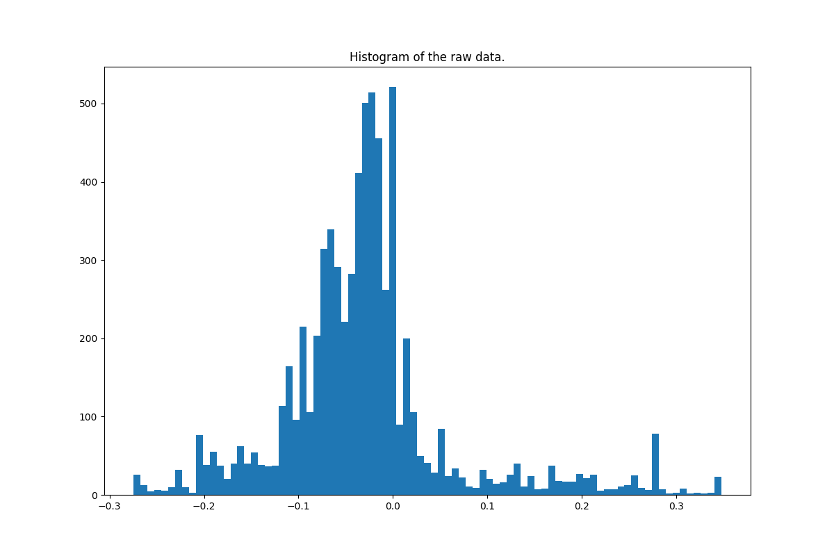
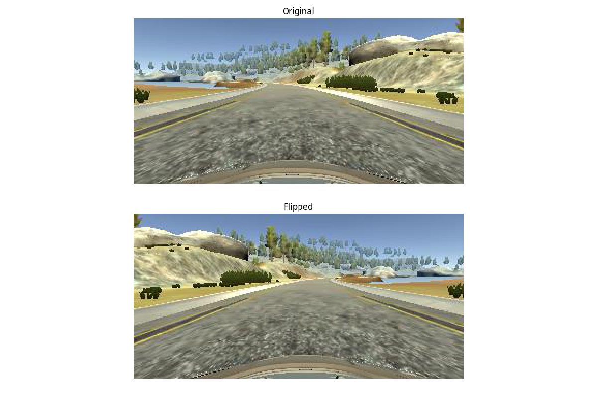
My approach was to have a 50% chance to flip the image horizontally so that it cancels that bias over a high number of iterations. The horizontal_flip(image, steering_angle): function outputs:

That enables the following more balanced histogram:

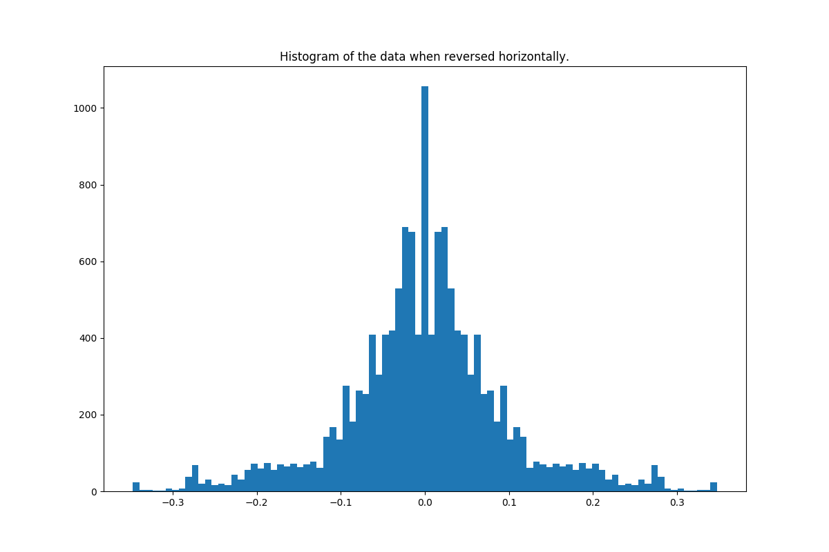
I obtain data that is heavily centered. At that point I decided to add the side cameras with a bias of 0.25. That number started at .2 and changed over time as I tested my models. The random_image_pick() function comes into play.

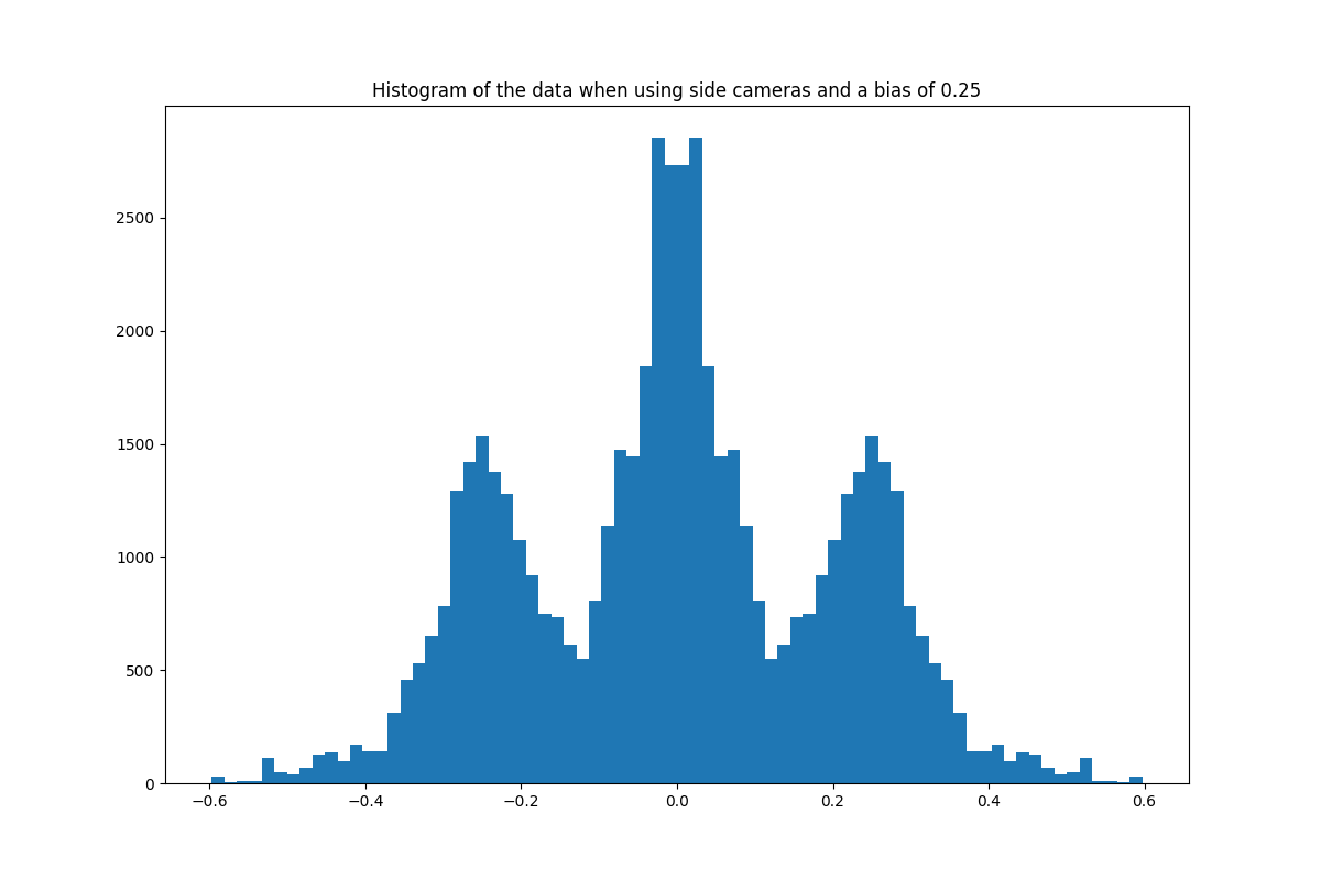
At that point, we can see that the data is strongly unevenly balanced and that causes problem for the model that learns to steer at values representing those 3 peaks more than everywhere else. I needed to balance my dataset. I introduced the following augmenting function:

def random_shift(image, steering_angle):
    '''
    Shifts the image horizontally and vertically
    '''
    X_range = 50
    Y_range = 10
    dX = X_range * np.random.uniform() - X_range / 2
    steering_angle += dX * .01
    dY = Y_range * np.random.uniform() - Y_range / 2
    shift = np.float32([[1,0,dX],[0,1,dY]])
    image = cv2.warpAffine(image,shift,(image.shape[1], image.shape[0]))
    return image, steering_angle

I obtain the following images:

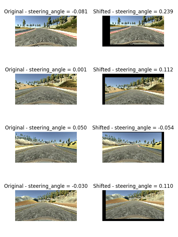
and the corresponding histogram when the data is shifted using that function. The data is directly obtained from the generator so that is represents well what the model is receiving.

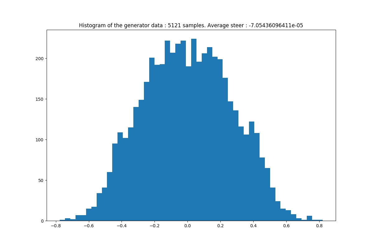
Lastly I wanted to test whether my model could generalize to the 2nd track. To do so, I needed to augment my images a little bit more. First because the 2nd track is very hilly. The model needs to learn to detect on the bottom and on the top of the image. In the random_shift(image, steering_angle): function, a vertical shift takes into account this.

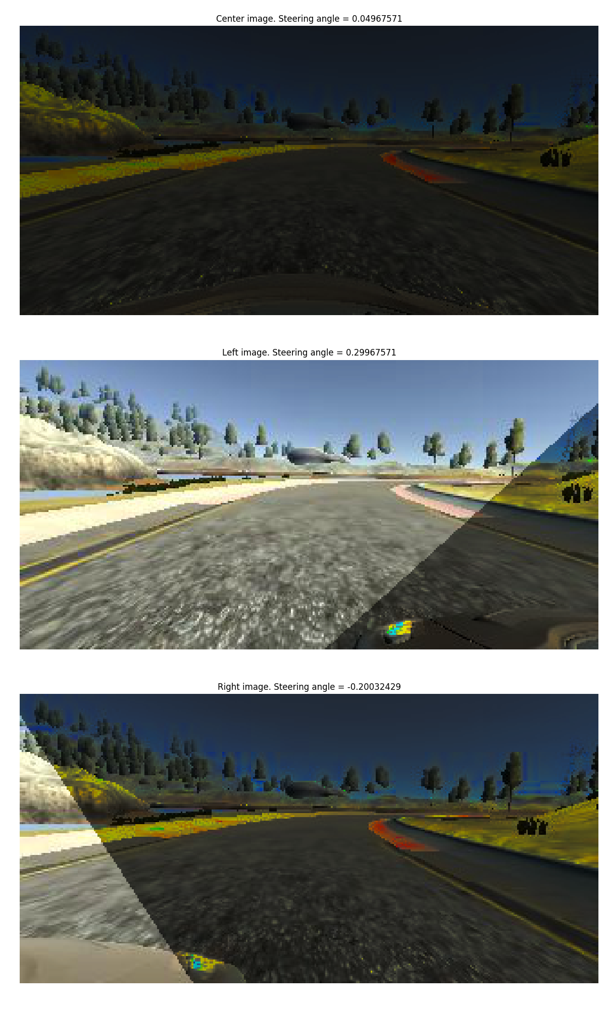
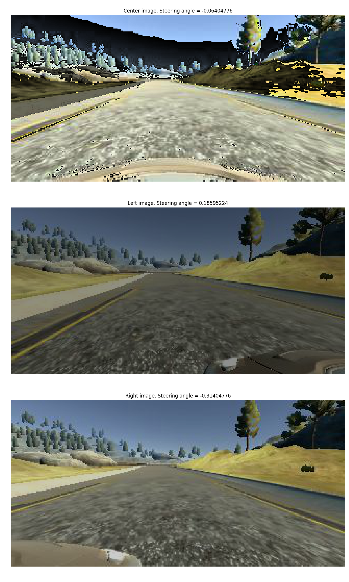
On the second track, the brightness is varying and in some places, shadows diminish the the luminosity quite significantly. I created the random_shadow(image): and random_brightness(image): to augment the training data even more. Here are the outputs to these functions.

Final Solution

1. Solution Design Approach

In order to gauge how well the model was working, I split my images and steering angle data into a training and validation set. With the augmenting functions, I believe I never experienced overfitting but in order to prevent it I introduced early stopping capabilities to the training process. If the validation loss doesn’t decrease after the following 2 training epochs, I rewind the model to keep the weights at that epoch.

This is done using the callback functionality provided by Keras.

earlyStopping = EarlyStopping(monitor='val_loss', patience=parameter['ESpatience'], verbose=1, mode='auto')

Here are my parameters that allowed an autonomous lap:

parameter = {'dropout' : 0.5,
              'model_type' : 'nvidia',
              'loss_function' : 'mse',
              'optimizer' : 'adam',
              'ESpatience' : 0,
              'reload_model' : 0,
              'steering_bias' : 0.25,
              'valid_over_train_ratio' : 0.15,
              'batch_size' : 128,
              'samples_per_epochs' : 40 * 128,
              'epochs' : 5,
              'color_augmentation' : 0,
              'shift_augmentation' : 1,
              ...
              }

2. Final Model Architecture

The final model architecture consisted of a convolution neural network designed by nvidia.

The activation functions are ELUs since the wrong outputs must be penalized. The way backpropagation is more effective.

3. Training Process

The final data distribution that I found would make the model work is the following:

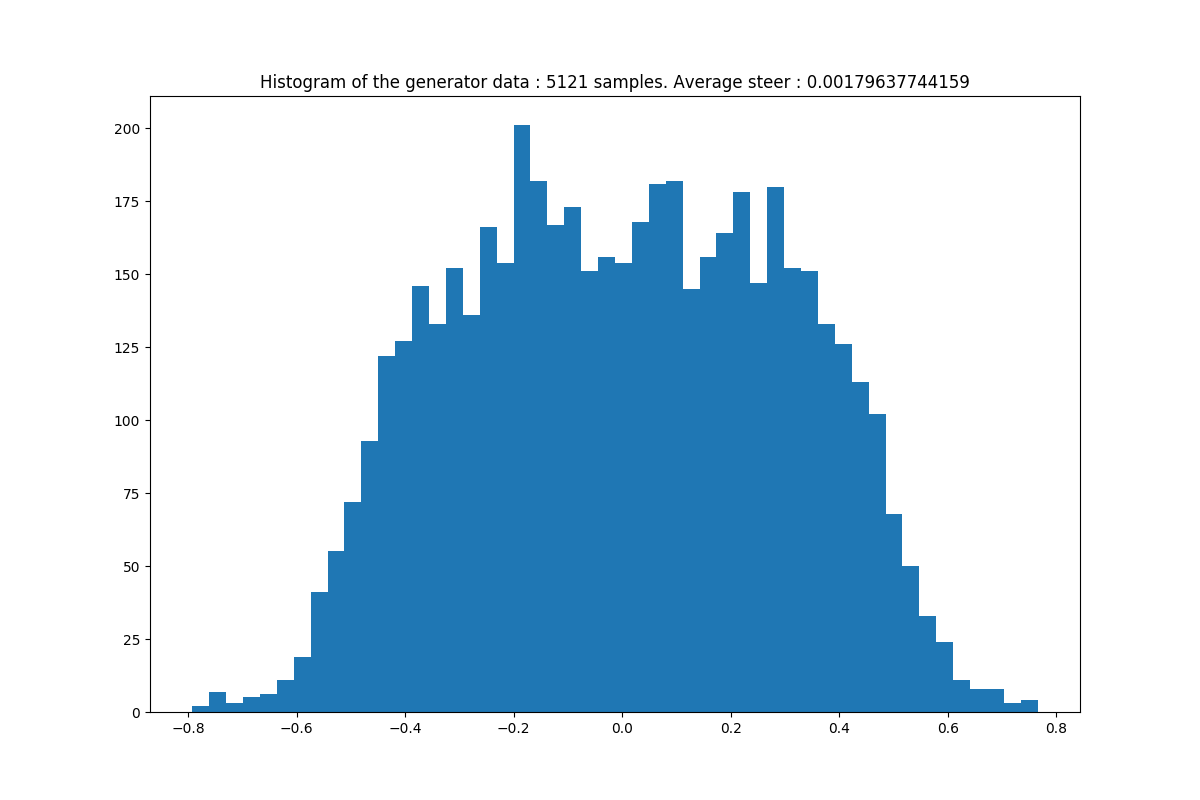
As a comparison to the last histogram higher in this file, this data distribution is more evenly distributed between -.25 and +.25. As a result, the car seems more responsive when a turn approaches whereas the previous one failed in the 2nd sharp turn after the bridge.

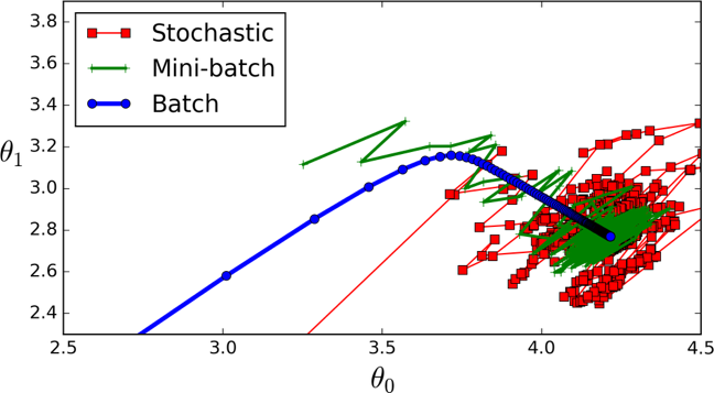
I opted for a mini-batch Gradient Descent approach with a batch size of 128. I trained my model in only 1 epoch.

4. Output video

I recorded an autonomously completed lap around the track one here

5. Improvements

• Obviously the car’s steering is not perfect and that should be fixed to prevent the fluctuation.
• Increase the model robustness so that the car can drive at full speed without leaving the track.
• Generalize to the second track. Currently, this model enable the car to drive on the second track for about 40% of the track without ever seen in the training set.

Network Visualization - Saliency Map

Visualization of what part of the image activates the neural net more than others.