Advanced Lane Finding Project
The goals / steps of this project are the following:
- Compute the camera calibration matrix and distortion coefficients given a set of chessboard images.
- Apply a distortion correction to raw images.
- Use color transforms, gradients, etc., to create a thresholded binary image.
- Apply a perspective transform to rectify binary image (“birds-eye view”).
- Detect lane pixels and fit to find the lane boundary.
- Determine the curvature of the lane and vehicle position with respect to center.
- Warp the detected lane boundaries back onto the original image.
- Output visual display of the lane boundaries and numerical estimation of lane curvature and vehicle position.
Rubric Points
Here I will consider the rubric points individually and describe how I addressed each point in my implementation.
Code Architecture
- I have my parameters in a separate file
parameters.pyso that they are gathered and I can tweak them more easily. - I my calibration code in
calibration.py. - In
test.pyis all my code for saving functions outputs for visual testing and filling in this report. - I wrote the main part of the algorithm in
detect.py.
Camera Calibration
Each camera have a particular lens that distort the captured image in a certain way compared to the reality. Since we want to grasp a view of the surroundings as accurately as possible, we need to correct this distortion. OpenCV provides some very useful functions to perform this task.
The code for this step is contained in the calibration.py.
I start by preparing “object points”, which will be the (x, y, z) coordinates of the chessboard corners in the world. Here I am assuming the chessboard is fixed on the (x, y) plane at z=0, such that the object points are the same for each calibration image. Thus, objp is just a replicated array of coordinates, and objpoints will be appended with a copy of it every time I successfully detect all chessboard corners in a test image. To do so I use the cv2.findChessboardCorners() function provided by OpenCV. imgpoints will be appended with the (x, y) pixel position of each of the corners in the image plane with each successful chessboard detection.
Here is an example of a successful detection:
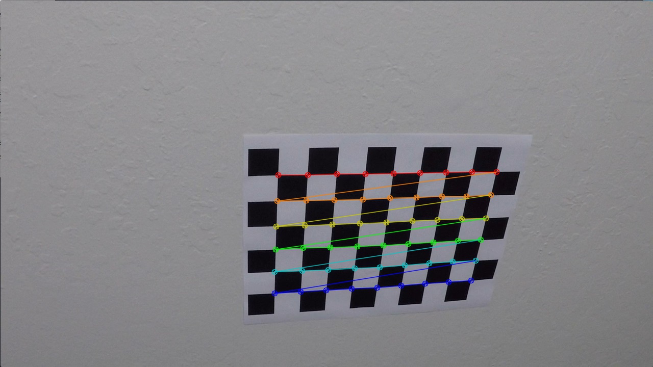
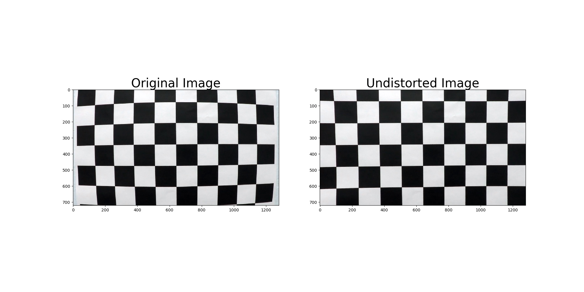
I then used the output objpoints and imgpoints to compute the camera calibration and distortion coefficients using the cv2.calibrateCamera() function. I applied this distortion correction to the test image using the cv2.undistort() function and obtained this result:
Pipeline (single images)
I am now going to describe the pipeline each images goes through in order to detect the lines. I am going to display images to illustrate each steps of the way.
1. Undistortion
The pictures of the chessboard were taken with the same camera as the one mounted on the car that took every pictures and videos that were provided for this project. Therefore, after calibrating the camera on the chessboard, we can use the same coefficients to undistort every images and videos of the road.
Since the calibration only needs to happen once, I store the results in a pickle file and load it whenever I need the calibration data.
import calibration as C
mtx, dist = C.LoadCalibrationCoeffs()
dst = cv2.undistort(img, mtx, dist, None, mtx)
LoadCalibrationCoeffs() can be called from anywhere after importing the calibration file.
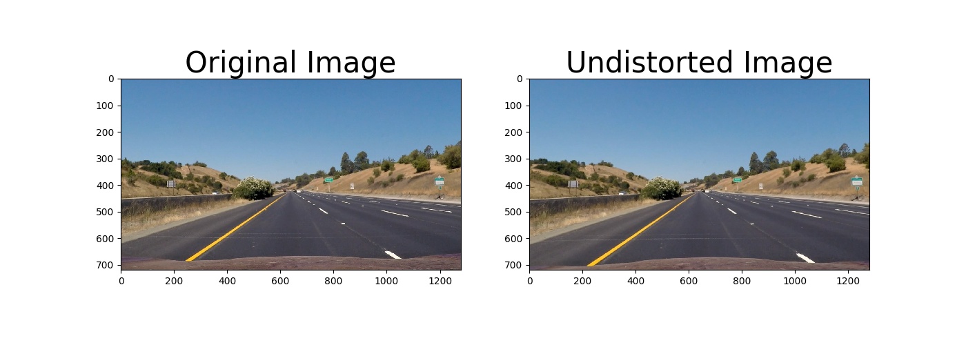
Here is the result after undistorting an image. The difference is subtle but we can see that the horizontal line at about y = 600 becomes seems more straight on the right image.
2. Lane detection
I used a combination of color and gradient thresholds to generate a binary image where every non-zeros pixels have a high probability of being part of a lane line.
a. Sobel operator
A Sobel operator is an edge-detection algorithm that computed and detect high gradient in a given direction by doing a 2-D convolution over the image. In this case, I chose to detect pixels which luminance (channel L of HLS color space) returns a high gradient in the x direction since the lines I am trying to detect are generally vertical in the image.
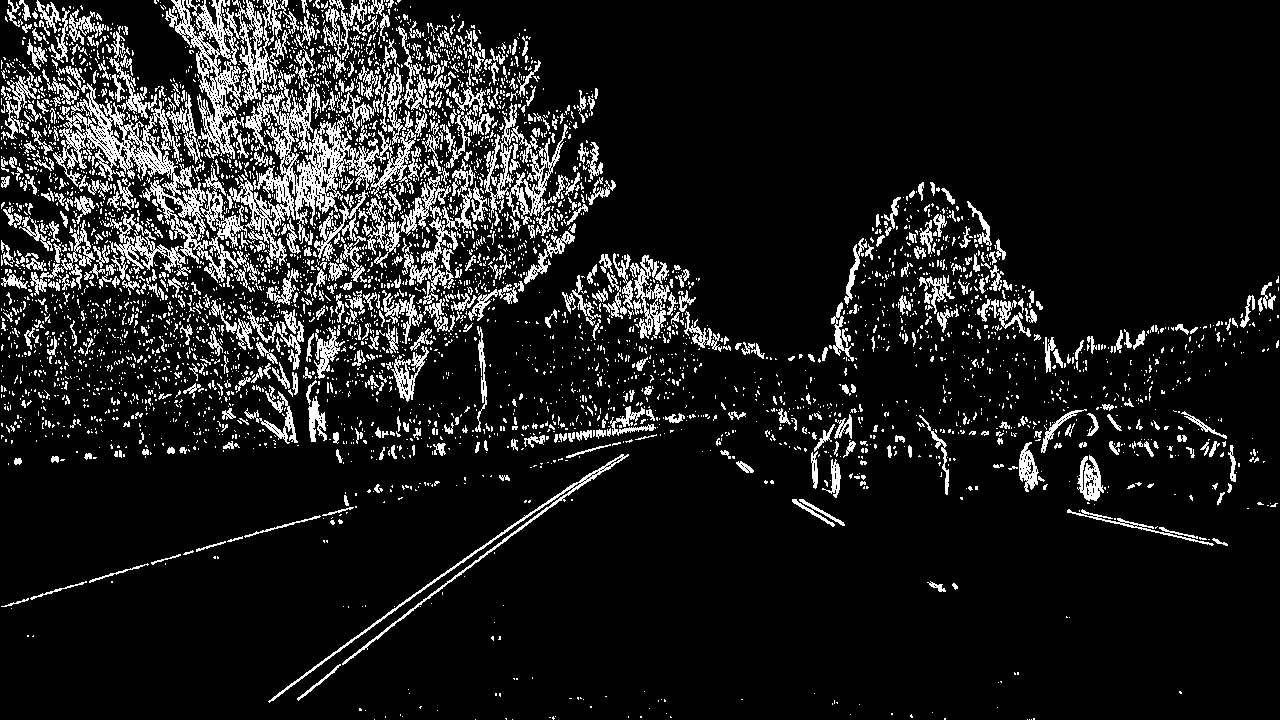
I chose the min and max thresholds for this function to be 20 and 100.
b. Color thresholding
Since the lines can be yellow and white, I chose to detect the lane lines by color as well. The S (Sue) channel of the HLS color space can be well suited for extracting a particular color.The following image shows how I extract the yellow lines:
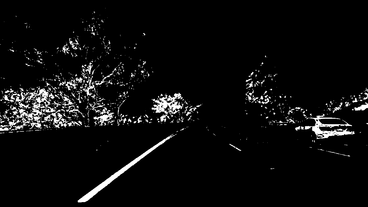
I found that extracting only the pixels between 170 and 255 would suit this problem quite well.
To extract the white color, I would chose the L channel and threshold between 200 and 255.
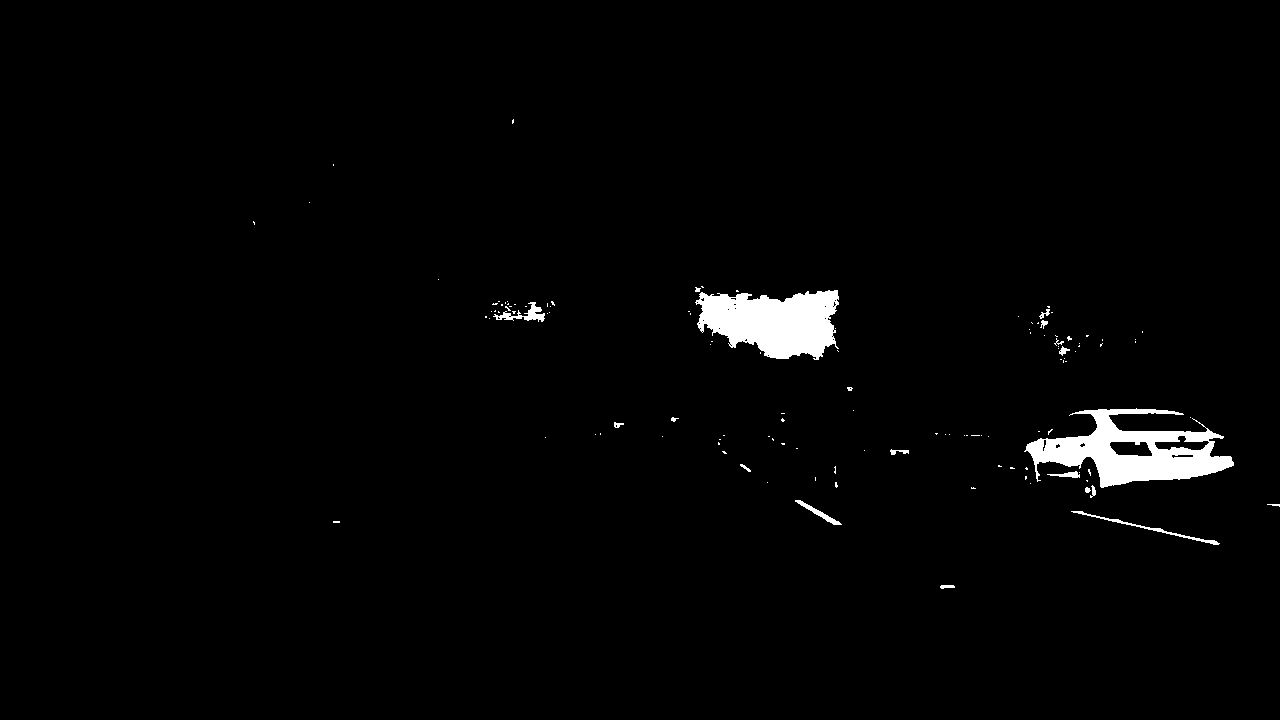
We can observe that the white detecting picture detect the right line more accurately.
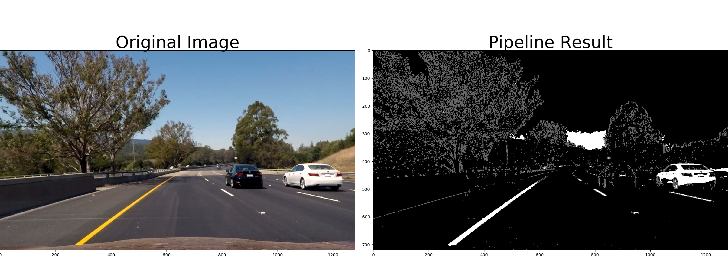
Final result
Here’s an example of my output for this step which is an aggregation of these previous steps.
3. Perspective Transform
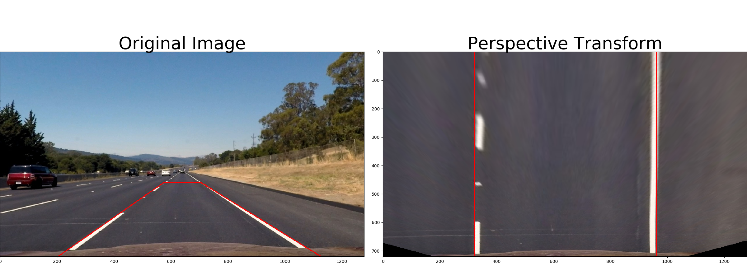
Since we want to detect the curvature of the lines, we need to change the perspective of the image. OpenCV comes very handy at doing so. I first delimitate the area in the image I want to transform and then define its destination shape. It can be observed by the 2 red rectangles I’ve drawn.
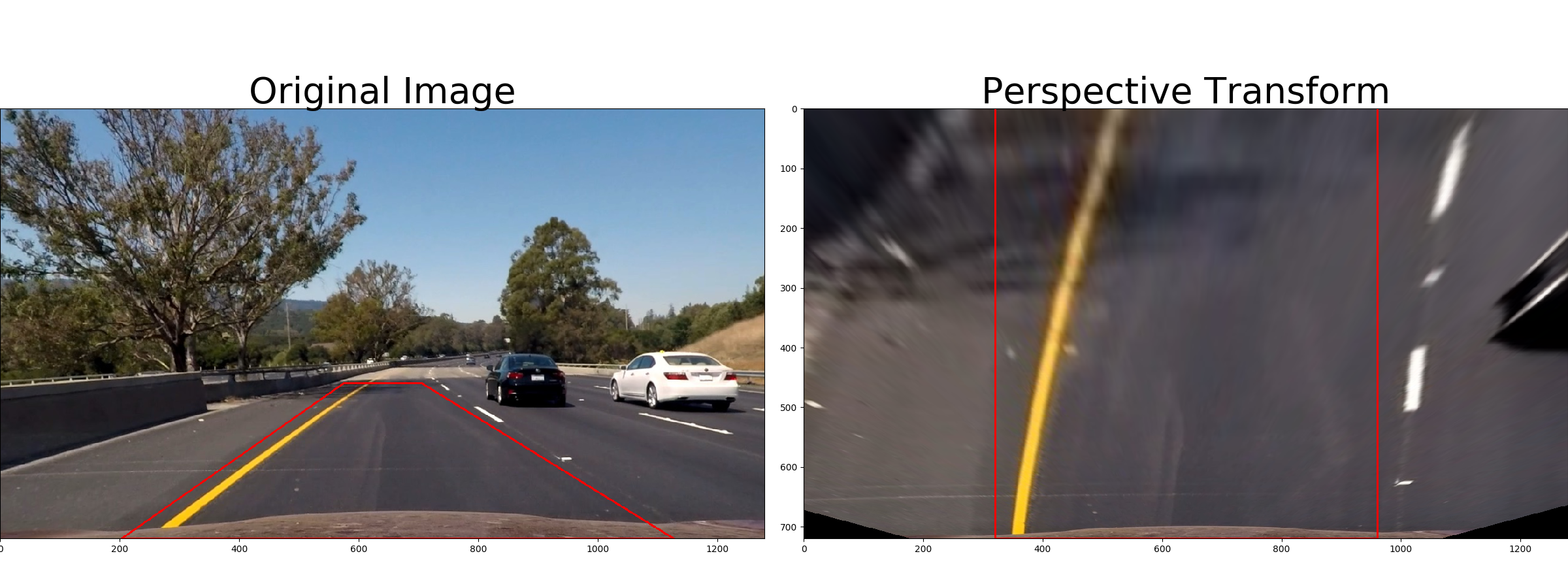
To obtain the right image I use the following function that performs a perspective transform:
def PerspectiveTransform(self, img, perspectiveMatrix):
    '''
    Change the perspective of the image
    '''
    return cv2.warpPerspective(img, perspectiveMatrix, (img.shape[1], img.shape[0]), flags=cv2.INTER_LINEAR)
The perspective matrix is computed by giving the coordinates of the 2 red rectangles.
I defined my points in my parameters.py file as :
parameters = { 'orig_points_x' : (575, 705, 1127, 203),#(617, 660, 1125, 188),
               'orig_points_y' : 460,
               ...
             }
and I construct my 2 rectangles that way.
def InitPerspectiveMatrix(img):
    '''
    Order of the points
            1 ---- 2        <- parameters['orig_points_y']
           /        \
          /          \
         /            \
        4 ------------ 3
    '''
    global src
    global dst
    src = np.float32(
        [[P.parameters['orig_points_x'][0], P.parameters['orig_points_y']],
        [ P.parameters['orig_points_x'][1], P.parameters['orig_points_y']],
        [ P.parameters['orig_points_x'][2], img.shape[0]],
        [ P.parameters['orig_points_x'][3], img.shape[0]]])
    dst = np.float32(
        [[(img.shape[1] / 4),     0],
        [ (img.shape[1] * 3 / 4), 0],
        [ (img.shape[1] * 3 / 4), img.shape[0]],
        [ (img.shape[1] / 4),     img.shape[0]]])
    #print(src)
    #print(dst)
    return cv2.getPerspectiveTransform(src, dst), cv2.getPerspectiveTransform(dst, src),
This resulted in the following source and destination points:
| Source | Destination |
|---|---|
| 575, 460 | 320, 0 |
| 705, 460 | 960, 0 |
| 1127, 720 | 960, 720 |
| 203, 720 | 320, 720 |
I verified that my perspective transform was working as expected by drawing the src and dst points onto a test image and its warped counterpart to verify that the lines appear parallel in the warped image.
4. Lane Pixels Identification
1. First frame
After obtaining the binarized image and transform its perspective to look at the road form the top, I need to decide which pixels belong to the lane. For the first image I compute a histogram of every pixels in the bottom half of image along the x axis and detect the 2 highest values on each sides. They give me the start of the lane.
Then, I iteratively create some bounding boxes (in green) and add the position of each pixels inside them to be part of the line. The center of the next box is the average x position of all of the pixels in the current box. That position is shown by the blue line.
At the end, I chose to color every pixels found for the left line in red and the ones for the right line in blue.
Here is the result:
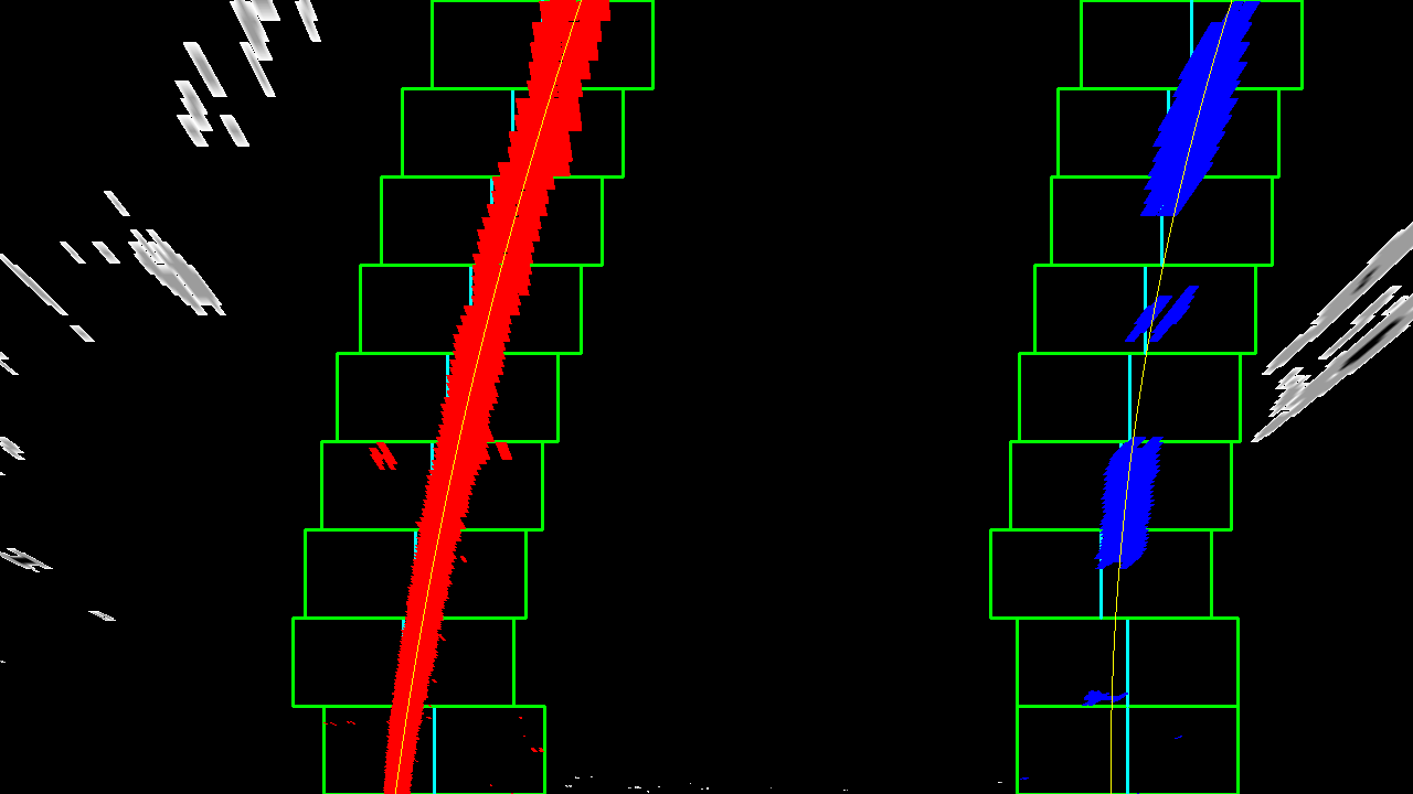
The yellow line in the middle of each lines are polynomials that are fitting each of the colored lines.
2. Subsequent frames
After obtaining both polynomials:
x = a * y^2 + b * y + c
I do not need to use the previous method that would be described as blind detection. I use the polynomials and only look at the area nearby.
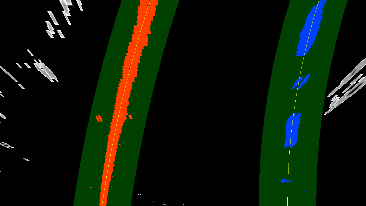
I extend each polynomials by a margin (50 pixels) on both sides, add every non zero pixels within that region and fit a new polynomial on top of that.
The code for that function is the following:
def DetectionFromPreviousPolynomial(self, binary_warped):
    nonzero = binary_warped.nonzero()
    self.nonzeroy = np.array(nonzero[0])
    self.nonzerox = np.array(nonzero[1])
    self.left_lane_inds = ((self.nonzerox > (self.leftPolynomialFit[0]*(self.nonzeroy**2) + \
                                   self.leftPolynomialFit[1]*self.nonzeroy + \
                                   self.leftPolynomialFit[2] - self.margin))
                         & (self.nonzerox < (self.leftPolynomialFit[0]*(self.nonzeroy**2) + \
                                   self.leftPolynomialFit[1]*self.nonzeroy + \
                                   self.leftPolynomialFit[2] + self.margin)))
    self.right_lane_inds = ((self.nonzerox > (self.rightPolynomialFit[0]*(self.nonzeroy**2) + \
                                    self.rightPolynomialFit[1]*self.nonzeroy + \
                                    self.rightPolynomialFit[2] - self.margin)) \
                          & (self.nonzerox < (self.rightPolynomialFit[0]*(self.nonzeroy**2) + \
                                    self.rightPolynomialFit[1]*self.nonzeroy + \
                                    self.rightPolynomialFit[2] + self.margin)))

    # Extract left and right line pixel positions
    leftx = self.nonzerox[self.left_lane_inds]
    lefty = self.nonzeroy[self.left_lane_inds]
    rightx = self.nonzerox[self.right_lane_inds]
    righty = self.nonzeroy[self.right_lane_inds]
    # Fit a second order polynomial to each
    self.leftPolynomialFit = np.polyfit(lefty, leftx, 2)
    self.rightPolynomialFit = np.polyfit(righty, rightx, 2)
5. Radius of curvature
The whole purpose of detecting a lane is to compute a lane curvature and from it a command to steer the wheel to control the car. The radius of curvature is computed at the bottom of the image, point closest to the car.
This is performed by the function
def CalculateCurvatureRadius(self, leftFitX=None, rightFitX=None):
in the detect.py file.
A useful link is the following.
6. Lateral position
Another very useful information is the lateral position of the car within the lane. It is obviously used to keep the car centered and prevent it from leaving the lane unintentionally.
To compute it, I measured the relative x position of the start of each polynomials.
def UpdateLateralLanePosition(self):
    '''
    Returns the position of the car away from the center of the
    road in meters. A positive value is on the right of center
    I am using the value at the bottom of the image of each fitted
    polynomial to evaluate the position of car compared to the
    lines. I am assuming the camera is mounted in the center of the
    windshield.
    '''
    roadCenter = (self.left_fitx[-1] + self.right_fitx[-1]) / 2
    # Conversion from pixels to meters using Udacity conversion data
    self.carPosition = (roadCenter - self.imageWidth/2)*self.xm_per_pix
    if (self.carPosition < 0):
        self.carSide = "Right"
    else:
        self.carSide = "Left "
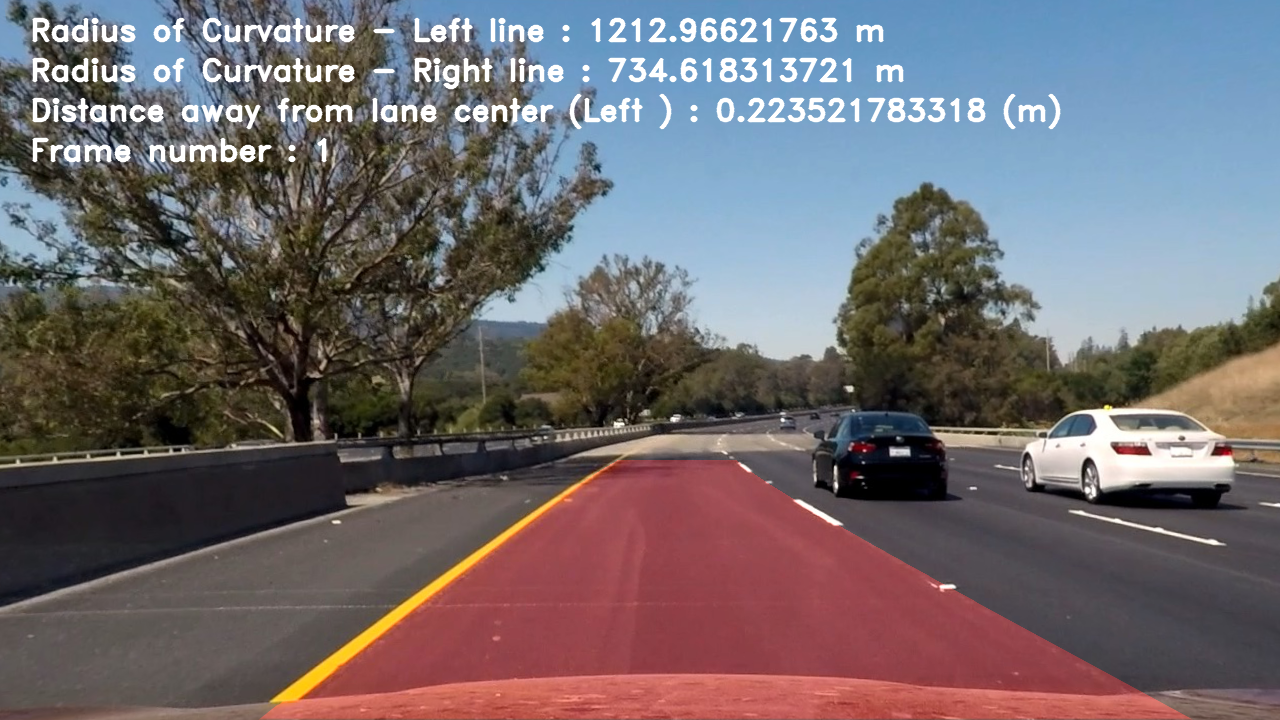
7. Final result.
For debugging and explanation purposes, I aggregated 4 different views as an output image.
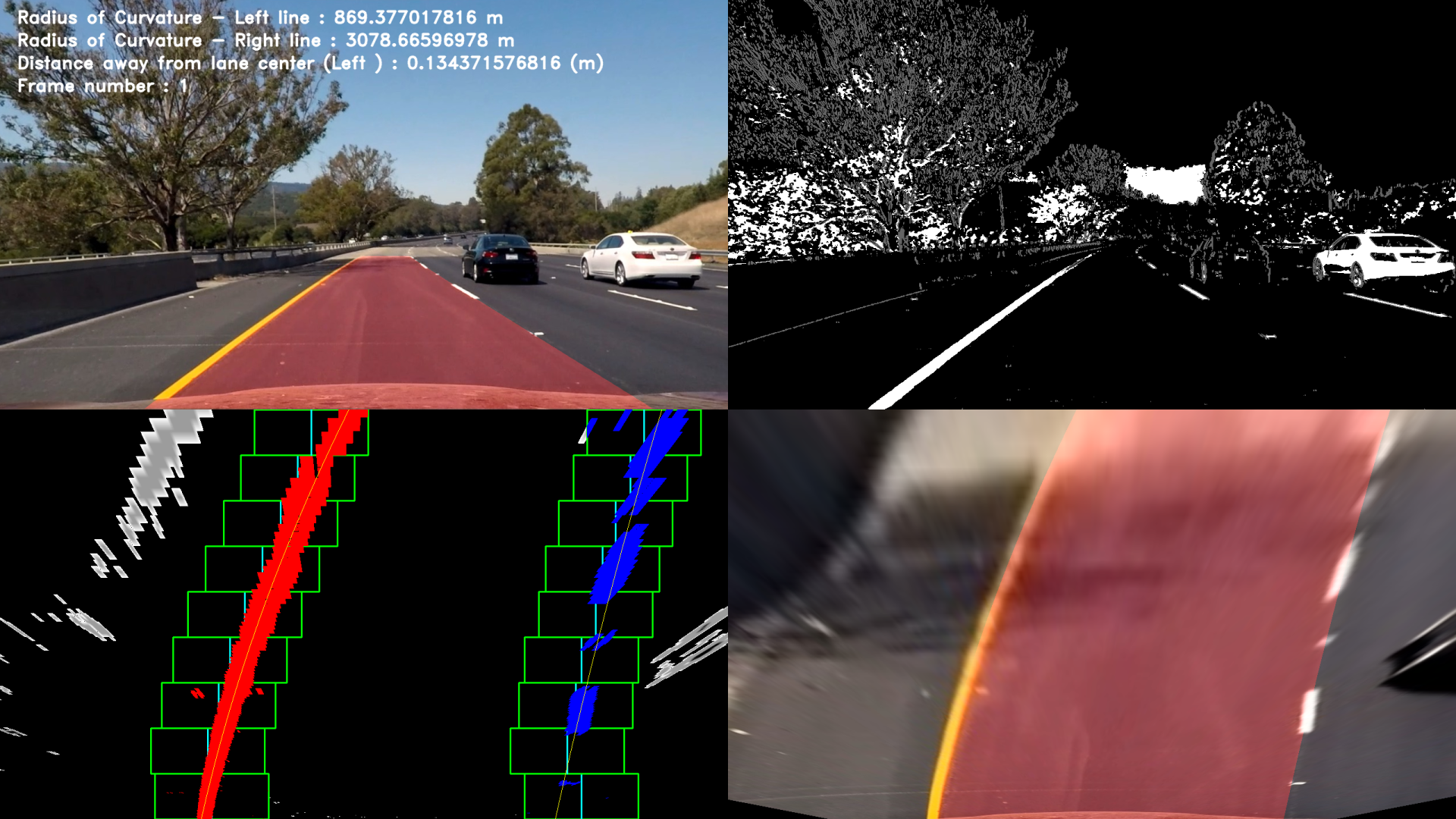
Here is a final result on a test image:
7. Conclusion
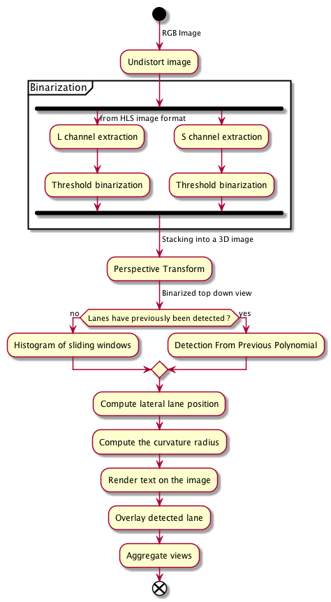
Here is a plantuml activity diagram of my pipeline:
Pipeline (video)
Now is the most interesting part, how does my pipeline performs on videos.
Here’s a link to the same result if you read this as a .md.
Discussion
The techniques I adopted for the solution I just presented work quite well with favorable conditions. It goes very wrong as soon as some other features of the road look a little bit like a lines. The detection would start considering them as well because I haven’t implemented a mechanism to check the accuracy the the fitted polynomial.
I could come up with some checking function that discards the polynomial if certain criteria are not met or if the curvature increase or decrease too rapidly for example.
Whenever the road would not be horizontal and the horizon line would either go up or down, the algorithm would go crazy. The distance up to which the algorithm should try to detect the road could be variable and adjusted with the car pitch from an IMU input.
